Exploring Algebra - Geometrically!

Stephen Arnold Compass Learning Technologies

A ladder leans against a wall. The top of the ladder overhangs the top of the wall.

The bottom of the ladder begins to slide steadily away from the base of the wall. What does it feel like at the top of the ladder?

Do you feel yourself going down steadily, or do you change speed on the way down?

An "Iron Man" race is organised at the local beach. The race begins from a buoy (A) located 2 kilometres from one end of the beach (O), and ends at the opposite end of the beach (B), which is 6 kilometres long.

I can swim at 4 km/h, and run at 10 km/h.

At what point (X) on the beach should I aim to land in order to maximise my chances of winning?

Two friends agree to meet during their lunch hour, but both are very busy and unsure whether they can make it.

They agree to wait for 15 minutes and, if the other has not arrived, to leave.

What is their chance of meeting?

How long should they wait if they wish their chance of meeting to be at least 80%? (adapted from NSW HSC Mathematics examination, 2005)

These problems are typical examples of investigative tasks which involve some elements of algebraic modelling. In each case, the central goal for the student is to generate an algebraic model of the situation, which will support deeper understanding and some measure of insight into the context, and perhaps even to provide the basis for prediction. A standard starting point for students in the case of such problems would involve them constructing a diagram by which they could gain some feel or understanding of the nature of the task, and perhaps some appreciation of the limitations: is the question realistic? Is the challenge even possible? For many years now, I have advised my students to begin with a piece of paper and to draw a picture before they begin the necessary algebraic manipulations required.

I have since realised that we have an ideal technological tool available for "scratching out" such models, in the form of the various tools for interactive geometry which have been available now for over a decade. Even more exciting, though, are the possibilities for a new type of tool - an integrated geometry and graphing environment. The wonderful, free GeoGebra, available for tablets, Windows and Macintosh from Geogebra.org, is such a tool. So is the exciting Texas Instruments TI-Nspire CAS, available for Windows, Macintosh, iPad and in handheld form, and which offers, not only integration of graphing and geometry, but lists, spreadsheets and the power of computer algebra!

The model offered by such tools goes well beyond that which is possible using a piece of paper. It is dynamic and capable of generating data which supports the building, first of a graphical model (from the data lists generated) and, then, an algebraic model by potentially replacing the numerical values for the variables in the sketch with symbolic values.

Using tools such as Locus and Data Capture, or simply having a partner record data points into a list, students are able to use their dynamic model to build a graphical picture, which will aid their understanding and interpretation of the problem situation. Even more importantly, it may be used to verify their attempts to build an algebraic model!
A great feature of *GeoGebra* is the ability to export your worksheet to an interactive web page, allowing students to access their work at home if desired! Double-clicking on the embedded web file brings up a full working version of the software to support further investigation, or the creation of new problem files. Again, this software does not care if you use tablet, Mac or PC!

In the case of the free version of Cabri Geometry now available for TI-83/84 series calculator (CabriJr), students may work in pairs, one generating data points from the model and the other entering these into list or spreadsheet facilities, from which graphical and then algebraic modelling may follow.

What is proposed here is a three-stage approach to algebraic modelling using these available tools:

From GEOMETRIC to GRAPHICAL to ALGEBRAIC!

Build a geometric model which includes a variable point, and the distance of that point from a point of origin. Measure also those other variables relevant to the question.
Collect data from the model, enter this into lists (either manually or automatically) and hence build a graphical model from this data.
Finally, build an algebraic model using the graph and the original geometric sketch – first, replace the numerical x measurement with a variable, and then from this build the remaining algebraic function. Verify it against the graph that was built from the geometric model.

In this way, students are constructing, not only sensible and cross-representational understandings of the problem situation, but at the same time building deep understanding of the key algebraic concepts of variable and functional relationships in a concrete and yet dynamic way.

The construction of such geometric models is non-trivial and requires some familiarity with the capabilities of the tool available. What follows is a brief step-by-step description of the process for the problems given, first using the simple CabriJr software, since this is likely to be the most readily available for classroom use right now.

Hold on to the Ladder

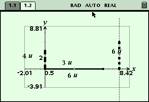
Most of these problems will begin with the construction of a segment, on which will be placed a point. Note that in these two simple, initial constructions, we embed a deep understanding of two critical concepts for all of algebra: the segment defines the domain (the actual values which it is possible for the variable to assume) and the movable point represents the variable. Actually, the true concept of variable comes into play when we measure the distance of the point from one end of the segment, which then becomes the origin. This needs to be drawn out in order to emphasise that, in algebraic terms, a variable always represents a numerical value!

Note that the length of the domain segment can be readily adjusted to fit the requirements of the problem (although this may not always be possible owing to limitations of the screen size).

In the case of the ladder problem, we next need to define a ladder. The trick here is that the length of the ladder should not change as it slides down, and this is easily achieved by creating a master ladder leaning against the wall in the garage, from which we will take the length of our actual moving ladder using the compass tool.

Construct a wall segment, then a ray which begins at our variable point and then passes through the top of the wall. Take the compass measurement from our master ladder, then centre it on the variable point to create a circle. Choose the point where the circle intersects with the line and create a segment from this back to our variable point. Now hide both line and circle to reveal our ladder leaning against the top of the wall, and able to be controlled by moving the variable point at the base.

Finally, measure the overhang of the ladder – the distance from the top of the wall to the top of the ladder. This will be our y-variable, related to the distance of the base of the ladder from the bottom of the wall. Using Automatic Data Capture, students should now generate data from the model and enter this into lists, from which the points may be plotted.

Some discussion should now follow concerning the limitations of the model. Perhaps begin by considering the question of domain – play with the model to see what happens when the base of the ladder moves too far away from the wall. How long should our domain segment be to be meaningful in this context? In fact, the domain segment should probably be no longer than the length of the ladder, since once the top of the ladder passes the top of the wall, it should fall straight down!

Limitations of the technology in terms of accuracy and even resolution may appear to be frustrations – but should be treated instead as teaching opportunities! They invite discussion and even the possibility of argument among the students – and any time you have your students arguing about mathematics in a mathematics lesson, you know you have been successful. In the end, these very inaccuracies cry out for an algebraic model. Numbers serve only to establish the possibility – we need algebra to establish any measure of certainty. Possibly for the first time in their school careers, your students may actually see the need for algebra!

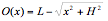
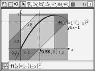
Return to the original geometric model, and replace the distance of the variable point from the origin with x. Let the length of the ladder be L and the height of the wall be H (or continue to work with the values of 6 and 4 for the moment). Students should see the application of Pythagoras' Theorem to the part of the ladder between ground and wall and build the functional expression for the overhang from this.

Or more generally:

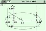
In fact, students then have the satisfying experience of graphing their functional expression (their algebraic model) and observing how closely it fits their data! This is a powerful modelling experience which builds deep understanding at the same time as it reinforces the value and usefulness of mathematics!

Of course, accompanying the entire process should be students attempting to put the problem into their own words! This is critical for understanding and for valuing what is being achieved. In this case, we are interested in what it actually feels like to be at the top of the ladder. As the base slides away at a steady rate, do you feel that you are falling at a steady rate? What does the model suggest? – clearly, the fall is not linear, but starts slowly and then speeds up!

Note, too, the possibilities for further investigation – especially with the support of computer algebra in TI-Nspire CAS.

A simpler form of this problem has the ladder leaning against the wall (not overhanging it). Build a new model and then try to put it all together since a real ladder should change from an overhang model to a leaning model once it reaches the top of the wall! For further study, what if the wall is leaning: no longer perpendicular to the ground – and our model is easily adapted to this!

Race along the Beach

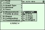
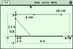
The beach race problem is easily constructed in a geometric environment and then involves some measurement and calculation.

Begin again with a domain segment (in this case, the length of the beach), and a variable point towards which the competitor will aim to land. A point out to sea from one end of the beach represents the start of the race.

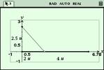
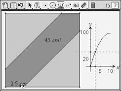
Measure the distance from start to landing point, and from this point to the end of the race. Together, these give the total distance covered in the race. In the example shown, I have set the starting point to be 2.5 kilometres out to sea from one end of the beach, and the beach to be 6 kilometres long. However, any values are acceptable since we wish to build towards a general algebraic solution.

The key to understanding this problem lies in realising that the solution occurs at the shortest possible time for the race, and time is the result of distance divided by speed. To give values for the two possible speeds, we create and measure two new segments somewhere out of the way (just as we created our master ladder hanging in the garage!) or simply use the Text Tool to type in the two numbers.

The total time taken for this race, then, will be the sum of the two times: that for the swim (distance from starting point to landing point on the beach) divided by the swim speed, PLUS the distance for the run (from landing point to end of the beach) divided by the run speed. Use the CALCULATE option to produce each of these times, and then add them together to give the total time for the race, as shown. It is useful to label these values with the Text Tool.

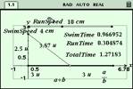
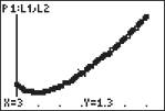
In this example, by aiming for a point 3 kilometres from the end of the beach, the time for the swim is 1.0 hours and for the run, 0.3 hours, giving a total time for the race as 1.3 hours. Pointing at each number and pressing the + key increases accuracy and the – key will decrease accuracy, as desired.

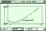
Enough points may be generated in this way to strongly suggest a non-linear model.

Back to the algebra to really understand what is happening!

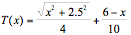
Let x represent the distance from the start of the beach, and with a little Pythagoras, we derive the following function for the total time taken for this race:

Any errors in the algebraic form (and there are likely to be errors as the students work towards a solution) will be immediately visible when the function graph overlays the scatter plot of the data. This is an experimental approach to algebra, in which the theoretical form is validated against the actual data gathered – a very powerful and convincing learning experience.

Traditionally, this problem leads to investigation of maxima and minima using calculus, and our modelling scenario is quite robust enough to provide a good basis for such further explorations. Using the power of a tool like TI-Nspire CAS, the algebraic scaffolding for such an investigation is readily available. The option to further explore these values using Lists and Spreadsheets is also available.

Meeting a Friend

Each year, the New South Wales Higher School Certificate examiners manage to come up with some really nice questions, and 2005 was no exception. The final question on the Mathematics paper was a fascinating blend of algebra, geometry and probability and a wonderful starting point for some algebraic modelling.

This question may begin as a geometric challenge for students, if desired: show them the square with the movable point on the base as shown, and challenge them to work in pairs to construct this model (noting that the triangles in top-left and bottom-right corners follow the movement of the variable point). Of course, building a square using interactive geometry is non-trivial, and much may be gained by challenging students to find multiple approaches using different properties of the square.
Building the bridge between the geometric and the algebraic is what makes this problem so special: using the Notes application within TI-Nspireallows the problem to be posed and scaffolded, and student thinking and answers to be recorded. The document created by the student solution offers a new path for teachers to follow student thinking and to evaluate their understanding.
The problem may be approached geometrically, building triangles which define the polygon, or algebraically by entering the inequalities specified in the question and observing the relationship to the square, as shown. Of course, it is absolutely essential that discussion should occur as to why the inequalities define this particular problem situation!
Using TI-Nspire CAS, it is possible to define the x-coordinate of the control point as a variable, say t, which can then be used in the inequalities to create a dynamic model. From this model can be built the graph which describes the various probabilities associated with different wait-times. Students may then build their algebraic model and verify it against the graph, providing very clear evidence that their algebraic approach is either accurate or otherwise! The power of the Lists & Spreadsheet to support students in their numerical investigations should not be underestimated,either. Strong multi-representational approaches to realistic problems lie at the heart of good conceptual understanding and positive attitudes.

The possibilities for such use of these wonderful tools appear great. Once again, appropriate technological tools encourage our students away from the role of passive spectators and into the driver's seat, as active participants in their study of mathematics, and algebraic modelling in particular.

Please feel free to visit Live Mathematics and STEM on the Web for more interesting problems and explorations.

[Special thanks to Professor Kaye Stacey from the University of Melbourne for the suggestion of the overhanging ladder problem!]