Getting Started with DataLogging in Mathematics
Stephen Arnold
Download in PDF format
The possibilities for using graphic calculators to enhance the teaching and learning of mathematics are great. However, the boundaries explode when these powerful devices are connected to data logging equipment: a whole new approach to mathematics learning becomes possible. Using real-world data to introduce the main functions (which are the bread-and-butter of high school mathematics) invites an experimental approach to the subject and encourages students to engage actively in their learning, as participants rather than as passive spectators.
The first five activities use simple data logging to introduce, in turn, linear (Activities 1 and 2), quadratic, hyperbolic and exponential functions. The last activity offers four different methods of producing a sinusoidal curve and so provides an introduction to trigonometric functions.
It should be noted that the motion detector (CBR™, or Ranger™) should be a mathematics teacherÆs best friend. It can be introduced from a very early age and used to enliven classes at any level. After introducing the main functions described here, there is value in having students attempt to simulate the various functions in turn using their own motion. Much will be gained as they experience for themselves the physical reality of each.
Learning Activity
Function Type
Data Source
1. Walking the line Linear Motion 2. Can you feel the warmth Linear Temperature 3. The Bounce Factor Quadratic Motion 4. Move into the light Hyperbolic Light, motion 5. Turn up the heat Exponential Temperature 6. Harmony all around Trigonometric Motion, sound, light
Learning Activity 1: Walking the Line
Top of Page
AIM To build student expertise in working with linear algebraic relationships, particularly with regard to gradient and y-intercept.
METHOD The use of a motion-detector is an excellent way for students to physically represent the algebraic concepts of gradient (speed of movement) and y-intercept (starting position).
PROCESS Begin with students informally moving in front of the motion detector, generating real-time graphs which the class should interpret. Attention should be drawn to the horizontal axis (time in seconds) and the vertical axis (distance in metres).
In the example shown, note that the motion began almost exactly 3 metres from the CBR™, and that the movement towards the sensor occurred for approximately 7 seconds.
Suitable warm-up activities include asking students (with help from class-mates where necessary) to make mountains and valleys (Do I start close or far away?), move fast and slow, towards and away from the source - all building student understanding of the concepts required to interpret such graphs. Some use of the Distance Match application (part of the Ranger™ program) will also help to build skills and understanding.
When students are sufficiently comfortable with the working of the device and the interpretation of the results, it is time to have someone again walk a simple straight line (like that shown above) and then quit the Ranger™ program, and turn on the graph grid (FORMAT: GridOn). Now the real work begins!
Explain that the task is to try and match a straight line (linear function) to the main part of the graph shown. Since this is a modeling task, it is usually a good idea to begin with the graph Y1 = X (as shown). How do we adjust the function to match the graph?
The trial-and-error nature of this activity is quite important: students learn more from their mistakes than from correct responses. Even with no background in this type of task, students will quickly discover the ideas of negative slope and y-intercept, and keep adjusting the values until they arrive at a result that most are happy with. While they should begin by counting the grid points to arrive at a ōrise over runö value for the gradient, students will quickly move away from the fraction to the decimal form, since this is more easily adjusted.
The Ranger™ program offers, from the opening screen, the option of three ōApplicationsö: distance and velocity matches, as well as a ball bounce program. The first of these provides a very useful introductory activity for students becoming acquainted with the concepts and skills involved here.
The Distance Match activities involve the calculator generating simple motion graphs, which students may then attempt to copy. As such, they provide a very suitable warm-up activity for further work.
It should be noted, however, that while the Distance Match is relatively easy, the Velocity Match is quite the opposite. It is very challenging and best reserved only for seniors or very capable junior students. Even teachers find this one hard, although if the attempt is made in a spirit of challenge, experiment and fun, it can be very worthwhile.
Learning Activity 2: Can you feel the warmth?
Top of Page
Top of Page
AIM To use real world data to introduce linear functions and lines of best fit.
METHOD Students use a data logger to gather temperature data in both centigrade and Fahrenheit units, then derive a line of best fit for the resulting plot.
PROCESS This simple experiment may be done in a normal classroom by simply bringing in some hot and cold water in cups.
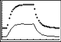
Set up the DataMate App and CBL2™ data logger with two stainless steel temperature probes in Channels 1 and 2. One should be set to read degrees Fahrenheit and the other degrees Centigrade. Set the time graph to read data at one-second intervals for 45 seconds.
Use a cup of cold water and another of hot water. Start data collection, holding the probes in the air for 5 seconds, then 20 seconds in the hot water and the remaining time in the cold water. Quit the DataMate App, and set the StatPlots to show L1 (time) against L2 (degrees Centigrade), and then L1 against L3 (degrees Fahrenheit). Use ZoomStat if desired to display the screen above.
Have students discuss what they observe from these graphs: the two curves are exponential, as temperature rises rapidly, and then falls away.
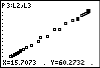
The power of this experiment for our purposes, however, arises when the calculator plots degrees Centigrade (L2) against degrees Fahrenheit (L3). Turn off the other plots, set up Plot3 as shown, then ZoomStat.
Students should discuss what they see: why is the line very close to being straight. Press TRACE and have students observe the motion of the cursor as it traces through the 45 seconds, but jumps around the graph screen. Explain what is happening.
This activity presents an opportunity for algebraic modeling, as the students attempt to fit a linear function to the plot.
Begin with Y1 = X, view the graph and vary the gradient and y-intercept until satisfied with the fit. This activity is always valuable, reinforcing understanding of gradient and intercepts and engaging students actively in the process.
If desired, students may be exposed to the regression lines available in the STAT -> CALC menu. Some discussion may occur when appropriate regarding the difference between median-median and linear regression lines. In this example, we would expect little difference between the two. Why?
Compare the values for this line with those arising from the data. Discuss the differences.
Finally, it may be worthwhile inviting students to simply enter the freezing and boiling points of water into lists as shown. Once again, set up a scatter-plot for these two points, and then compute the line of best fit using one of the linear regression options available under STAT -> CALC.
Learning Activity 3: The Bounce Factor
Top of Page
AIMĀĀĀĀĀĀĀĀĀĀĀĀĀĀĀ To build student expertise in working with quadratic algebraic relationships, based upon real-world data.
METHODĀĀĀĀĀ This is a simple activity in which students generate quadratic data using the motion detector in two different ways.
PROCESSĀĀĀĀĀ This activity may begin with the throwing of a soft ball or other suitable object to and from students around the room. Draw their attention to the path of the motion, and have them sketch this motion on a pair of axes.
Next have students try to model that motion themselves by moving in front of the CBR™. Invite discussion and contributions from others in order to try to improve the graphs produced. This activity quickly reveals the nature of student understanding regarding parabolic motion. Particular attention should be drawn to the different units being used in both situations. Their first sketch graph will have displacement on both axes, horizontally and vertically. The motion detector captures time on the horizontal axis and displacement on the vertical. Although both graphs may look similar (and certainly both are parabolic), they are measuring quite different things.
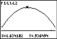
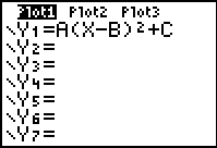
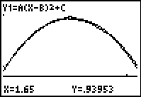
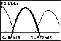
Finally, conduct a ball bounce experiment, using the motion detector. Each bounce is an inverted parabola. Have students isolate one of the parabolas and attempt to match a quadratic function, taking note of such features as the coordinates of the maximum turning point. Suggest the use of the quadratic form Y = A(X ¢ B)2 + C as the basis for their model, and have them record from their graph the coordinates of the turning point, as shown.
A little trial and error with the values for A, then, leads to a good model for the motion. Changing the viewing window allows students further practice as they repeat this exercise for the other parabolas available from the ball bounce.
This activity brings with it another bonus. If the ball bounce is carefully recorded, the high points of each parabola actually decrease exponentially: students should verify this, both by modeling, but also by observing that the ratio of consecutive terms in such a sequence should be (fairly close to) equal! This ōbounce factorö could be measured for a variety of different balls ¢ in the example shown, the bounce factor was around 0.9, making it most suitable for this activity.
Learning Activity 4: Move into the Light
Top of Page
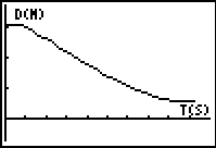
AIMĀĀĀĀĀĀĀĀĀĀĀĀĀĀĀ To model motion which is hyperbolic in form from real-world data.
METHODĀĀĀĀĀ This is a simple activity in which students generate data using both light probe and motion detector.
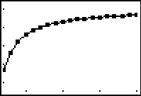
PROCESSĀĀĀĀĀ Using a CBL2™ data logger, DataMate App and both CBR™ and light probe, students may gather data on light intensity as a function of distance from the source. This experiment is best done in a darkened room with a strong light source, such as an overhead projector.
Once again, students should begin by estimating what they think the graph of the light intensity will look like. Will it be linear? Positive or negative gradient? If not linear, then what should we expect in the curve?
Discussion should lead to the recognition that the graph should be hyperbolic. This is a graph of distance against light intensity. Attention should be drawn to the natural behaviour at the extremes: what is happening when distance is zero? As distance from the light source becomes large?
The graph shown was produced by simply moving the CBL2™ and probes back and forth in front of the light source over a 5 second interval. The hyperbolic nature of the curve may be clearly seen, but if the graph is TRACEd, then the actual nature of the motion will be revealed through the sequence of points jumping back and forth rather than following the line of the curve.
The fact that the function being modeled is actually the square of the hyperbola (of the form 1/x2 rather than 1/x does not detract from the value of this activity. The properties of the two functions are sufficiently similar that the main features are preserved.
Students should be given a variety of situations which may be modeled hyperbolically: such practical situations as the effects of price upon ticket sales, or the effect of the number of workers upon the planting of seeds lead naturally to hyperbolic functions. Experience with real-world examples will help students to feel confident in their dealings with such functions.
Learning Activity 5: Turn Up the Heat
Top of Page
AIMĀĀĀĀĀĀĀĀĀĀĀĀĀĀĀ To model the exponential function using real-world data..
METHODĀĀĀĀĀ Students use the data gathered from a previous activity (Data Learning Activity 2: Can you feel the warmth?) to investigate the properties of exponential functions.
PROCESSĀĀĀĀĀ In this previous activity, students used two temperature probes together to collect data in both degrees centigrade and degrees Fahrenheit. Here we only need one of those sets of data ¢ it does not matter which, but for convenience we will use degrees Centigrade.
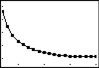
The experiment consists of measuring the air temperature first for approximately 5 seconds, then 20 seconds into hot water, followed by another 20 seconds in cold water. Using the WINDOW menu, it is a simple matter to focus on the last section of data, between approximately 25 and 45 seconds, as shown.
This data provides an excellent exponential model which students should observe, discuss and, eventually, attempt to model. The actual finding of correct figures for this model is not the important part of this activity. Rather, it is the process of becoming familiar with the effects of the various parts of the exponential function that drives it. Beginning with a model of the form a x bc ¢ x + d students in small groups are free to experiment with different values in search of a reasonable fit.
Having attempted this activity, a follow-on exercise would involve doing the same for the data from the first part of the graph: from 5 to 25 seconds, giving the plot shown. Again, the real point of this exercise is the discussion that should ensue concerning the properties of the function and those of the real-life situation, which gave rise to the data.
Learning Activity 6: Harmony All Round
Top of Page
AIMĀĀĀĀĀĀĀĀĀĀĀĀĀĀĀ To model the sine function using real-world data.
METHODĀĀĀĀĀ Using a plastic ōslinkyö students model a simple harmonic motion to introduce trigonometric functions. (If a slinky is not available, swinging a handbag or any object suspended from a string will work).
PROCESSĀĀĀĀĀ Initially, students should observe the motion of the slinky and attempt to draw the graph for themselves.
This activity is very simple: set the Ranger to 5 seconds, activate using the trigger, detach and lay it on the floor. While one student operates the slinky (more than 0.5 metres above the device) another activates the trigger when the motion is stable.
Once again, much will be gained by students using trial-and-error techniques to match a curve as closely as possible to the data. When the class is satisfied with their efforts, then the SinReg option (STAT->CALC) will reinforce and assist in the process.
Of course, another simple motion detector activity here involves students on swings ¢ a wonderful excursion for seniors, who will physically feel the motion: when the velocity is zero, and when it is at a maximum ¢ even when the force (or acceleration) is acting (downwards!).
Two ways to test how good a trigonometric function you have collected:
- Check out the Velocity-Time graph for the motion. It should be regular and clear, as in the first graph below.
- Plot Distance (L2) against Velocity (L3) and see how close to a circle your motion is. This one is a bit surprising and very interesting for students to discuss ¢ hence the name ōcircular functionsö!
ĀĀĀĀĀĀĀĀĀĀĀ
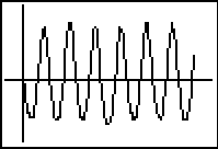
The two sinusoidal curves shown below are derived from two entirely different sources. The data for the first is collected using a microphone probe, with someone singing a clear steady note. The settings are the default settings chosen by the DataMate App when it senses the microphone probe, collecting 200 samples at intervals of 10-4 seconds (1000 samples per second), hence the experiment only lasts for 0.2 seconds.
The second set of data is generated by holding a light probe underneath a fluorescent light, with the same sample rate and time. While this works best in a darkened room, it should work effectively in most classroom situations where there is not too much background light. Interestingly, this curve involves the absolute value of a sine (or cosine) function, as the data logger collects, not a smooth continuous effect, but the flickering on and off of the light source at the standard rate of 50 cycles per second.
Again, students should attempt to match the curves manually, working in pairs or small groups to encourage verbalization: they need to put their thoughts into words and to share these with others to get the most out of such activities.
Students need, too, to attempt to relate the real world situation to the features of the mathematical function, with particular focus upon the key concepts of domain and range, and those characteristics that define each of the function types studied.
Mathematics was never taught like this when I was at school! If such an approach blurs the lines a little between mathematics and science, then so be it. Mathematics may be an activity of the mind, but the marvelous ways in which it models our real world are too many and too important not to be used to advantage. Activities like those described here, if used well, build both deep understanding and skills at the same time.
Consider the possibilities.