©2018 Compass Learning Technologies ← Live Mathematics on the Web →Bezier Curves
Introducing Bezier Curves
With thanks to Jon Roberts
For a step-by-step introduction using TI-Nspire, work through the Bezier Intro and download the TNS file.
Most of the curves you see on a computer screen or printed page - everything from text fonts to animations - are generated mathematically using Bezier Curves (sometimes called Bezier Splines).
Two GeoGebra examples are shown here - a quadratic bezier (controlled by points A, B and C) and a cubic bezier (controlled by all four points, A, B, C and D).
Drag the control points around and see the effect this has upon the curves.
Input:
CAS Input:
CAS Output:
These curves have been generated geometrically. The Dilation Transformation is used to set points which move in proportion to the point P on segment AB. This is interesting and powerful mathematics, but the real control comes when the curves are generated algebraically.
This may be done in several ways, but one relatively easy way involves using recursive formulae, beginning with one like this:
bezier(a,b,t) = a*(1 - t) + b*t
Suppose a and b are two numbers (say, 1 and 5). What happens as the value of t varies between 0 and 1?
When t = 0, the formula is completely "a" and when t = 1, it gives "b". For values between 0 and 1, it gives values between a and b, just like dragging a slider point P between the points A and B on the figure.
Then explore the second order bezier function,
bezier2(a,b,c,t) = bezier(a,b,t)*(1 - t) + bezier(b,c,t)*t
Use GeoGebra to explore! In the window above, copy and paste these two definitions into the Input Bar.
bezier(a,b,t) := a*(1-t) + b*t
bezier2(a,b,c,t) := bezier(a,b,t)*(1 - t) + bezier(b,c,t)*t
Now you might use GeoGebra's Computer Algebra System - tap the menu icon in the top right corner, choose Perspectives and CAS or just use the CAS input field above - NOTE: the first time you use this you may need to tal a couple of times to give time for the CAS engine to warm up!
Now for our example, the x-coordinates for A, B and C are 3, 1 and 5, so try the command bezier2(3,1,5,t). press the CAS input button a couple of times to see the result.
For the y-coordinates, try bezier2(5,2,-1,t)
Can you see how this might relate to our figure?
In general, we could define x and y coordinates in GeoGebra using x(A) and y(A), and so try bezier2(x(A),x(B),x(C),t) and bezier2(y(A),y(B),y(C),t).
What if we used parametric equations? Select the Geogebra window above and use the Input Line to enter (bezier2(x(A),x(B),x(C),t), bezier2(y(A),y(B),y(C),t)).
Is this what you expected?
You can also use the form Curve(bezier2(x(A),x(B),x(C),t), bezier2(y(A),y(B),y(C),t),t,0,1)
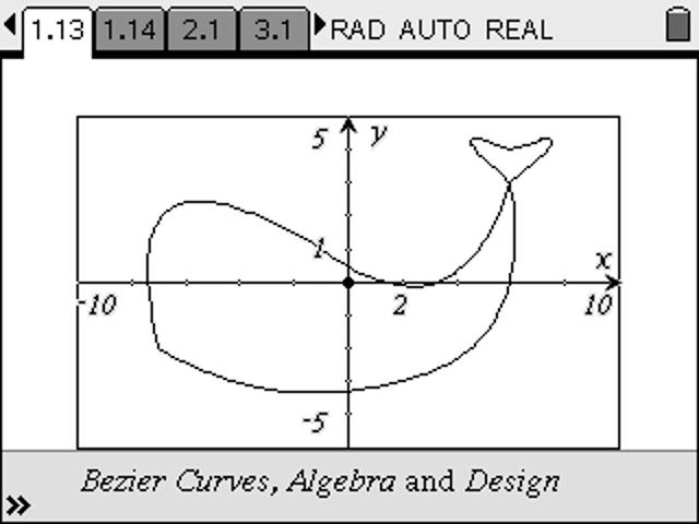
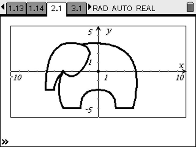
The possibilities for exploring interesting mathematics are great - with even the chance to display some artistic tendencies along the way!
Now what about that cubic curve?
Steve Arnold, Created with GeoGebra
©2018 Compass Learning Technologies ← Live Mathematics on the Web ← GeoGebra Showcase